Inference latency for open-source models has dropped rapidly in recent months, with providers offering increasingly fast endpoints. We wanted to bring that focus on speed to specialized models running on local hardware. FPGAs offer an interesting midpoint between GPUs and ASICs (low power, low latency, and avoiding the necessity of a tapeout), and we wanted to see how fast we could make a language model run on an FPGA.
On an AMD Kria KV260, we ran a transformer with roughly one million parameters at around 10,500 decode tokens per second.
The model's weights and attention cache fit entirely in the FPGA's on-chip memory. Realistically, this is the ideal way to operate such models on an FPGA, since storing weights in DDR for larger models causes latency to rise dramatically. Once loaded, the FPGA executes the transformer part of the model, while the board's ARM processor handles tokenization, control, and text output.
The result is a machine that writes children's stories:
Once upon a time there was a little robot. He was very cheerful and loved to play with his friends. One day, the …
Model architecture
The model
We started with shibatch/tinybpe1m, a pretrained, decoder-only Llama-style transformer with 935,040 parameters. The model has four transformer blocks, a hidden width of 128, a feed-forward width of 352, and two attention heads. Its vocabulary contains 512 tokens, and our implementation supports a total context of 256 tokens.
Here’s the architecture:

The model was trained on TinyStories, so it completes simple stories based on the input. We kept its architecture and tokenizer and focused on a working FPGA implementation and making inference faster.
Model weights
The original FP32 parameters occupy 3.74 MB. To shrink them, we quantized the matrix weights to four bits, with one FP32 scale for every group of 32 weights. The exported parameters occupy about 0.59 MB, a 6.36× reduction.
That makes it possible to keep the weights alongside a ~1 MB attention cache, which stores keys and values from earlier tokens. The weights and cache live in UltraRAM, while smaller arrays, including scales and normalization weights, use BRAM. Keeping this data on-chip removes the need to fetch model weights from DDR at every decode step. DDR still handles the initial upload and input/output transfers.
Latency optimizations
Mixed-precision processing
The matrix engine uses the Q4 weights together with dynamically quantized INT8 inputs. These inputs are the intermediate activation values flowing through the model. Because they change as the model processes tokens, we calculate their scales and convert them to integers as needed.
For a single multiplication:
While in this example the scaled result matches the original multiplication, in general, quantization can introduce rounding error. For a matrix product, the hardware adds the integer products within each group, then applies the corresponding scales.
Attention, normalization, rotary positions, nonlinear functions, residual additions, and the attention cache remain FP32, implemented in FPGA logic. Those operations could also be converted to fixed point for faster inference, but we kept them in FP32 for this experiment so we could focus on scheduling and data movement.
Decoding in one batch
Our initial implementation sent all 512 output scores, or logits, from the FPGA back to the ARM after every decode step. The ARM selected the next token and launched another FPGA command. That repeated handoff introduced avoidable overhead.
We instead moved the greedy decoding loop into the FPGA, where it runs the decode steps, picks each next token internally, and returns the completed token sequence at the end.
Attention optimizations
Attention lets the current token draw information from the context. For one head in one layer, the model computes a query vector for the current position and compares it with the key vector at each context position . Those comparisons determine how much each position's value vector contributes to the result. Each vector in this model's attention heads contains 64 numbers.
With context positions, including the current one, we compute the scores, attention weights, and output as follows. The dot product is divided by :
The dot product multiplies the 64 corresponding components and adds the products. Softmax converts the scores into positive weights that sum to one; subtracting the maximum score keeps the exponentials numerically stable. Both sums run over all context positions. The output is a weighted mixture of their value vectors, which the rest of the transformer processes before predicting the next token.
The KV cache saves earlier keys and values so we do not have to recompute them. Each new query still needs to read those keys and combine the values, however. As the context grows, each decode step has more cached data to process.
Our first optimization addressed how that work was scheduled. An arithmetic pipeline overlaps calculations at different stages, allowing new work to enter before earlier results have finished. The original code ran a short pipeline for each cached key: read its components, calculate partial dot products, wait for the results, and combine them before advancing to the next key. Although the inner loop could accept work every clock, repeatedly filling and draining it added overhead.
We changed this into a continuous scan across the cached keys. An 8 KiB banked BRAM buffer holds partial dot products, which a separate pass combines into scores. This lets the key-processing pipeline keep accepting work across successive keys while preserving the original summation order. The buffer is reused for the next head; softmax and value mixing remain separate stages.

Along with changes including wider cache access, we reduced the reported maximum attention-function latency from 39,074 to 4,382 cycles. These are HLS compiler schedules; decode throughput was measured separately on the board.
Matrix and scheduling optimizations
We widened the matrix engine from 64 to 256 parallel integer products per iteration. The final version processes two output rows together, using four dual-port memory banks to supply the necessary weights and scales. This change also exposed a compiler regression. We used bounds checks for a possible odd final row, which ultimately prevented HLS from flattening the loop into the intended pipeline. HLS reported a matrix-function upper bound of 20,310 cycles—well above our 1,000-cycle target.
Hardware and performance
The final design meets a clock target of approximately 200 MHz, or one clock cycle every 5 ns. Its nominal platform clock is 199.998 MHz.
The placed design, including the platform and kernel, uses:
| Resource | Used / available | Utilization |
|---|---|---|
| DSPs | 496 / 1,248 | 39.74% |
| BRAM tiles | 124 / 144 | 86.11% |
| UltraRAM blocks | 46 / 64 | 71.88% |
| LUTs | 84,024 / 117,120 | 71.74% |
| Flip-flops | 103,889 / 234,240 | 44.35% |
The finished design delivers about 10.5k decode tokens/s, excluding model loading and prompt processing. In a separate on-board latency measurement, a warm 32-token request reached its first visible generated text in 7.491 ms and completed in 7.632 ms, both medians. Those times are close because the output arrives as a batch. Browser and SSH transport add their own latency.
There’s room to go faster. The design uses about 40% of the DSPs, but already consumes 86% of the BRAM tiles and 72% of the LUTs. More arithmetic will need memory ports and routing to support it. The next useful optimization will depend on which resource actually holds up the loop.
Debugging with HyperBench
We brought the regressed source into HyperBench to investigate the slowdown. We connected the project’s GitHub repo as well as two hardware stations: an EC2 instance running Vitis/Vivado, and the KV260, reached over SSH. EC2 handled compiler runs while the board connection provided access to programming and inference operations.
For each hardware station, we supplied a scaffold describing its tools and available operations, then asked HyperBench (HB) to generate an adapter. Then, we reviewed the generated code, ran validation on the station, and enabled it. This way, HB could call the necessary tools on each hardware platform as needed.
Using HB Discover, we investigated the matrix function slowdown, with checks requiring successful synthesis, an estimated clock period within the 5 ns target, and a matrix-function upper bound of no more than 1,000 cycles. The initial run containing the slowdown reported 20,310 cycles for the matrix function, which resulted in only around 850 tps when running on an FPGA.
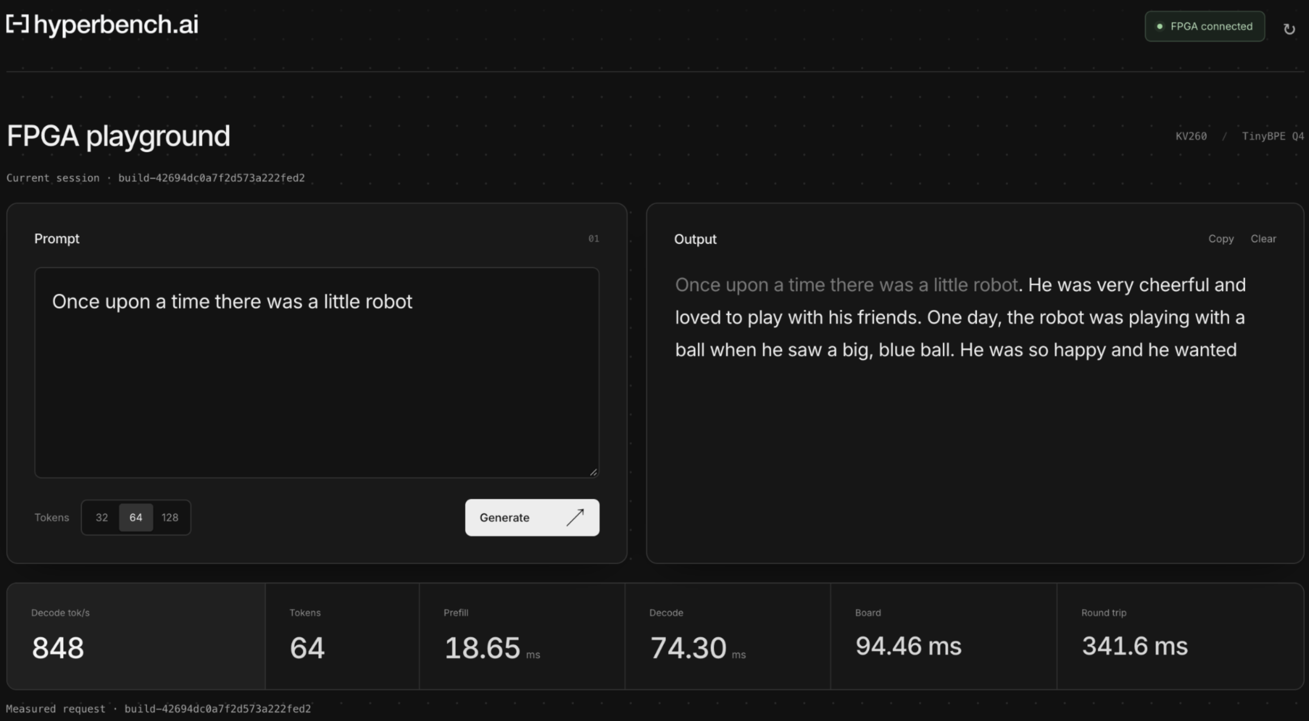
Once the regression was detected, we used HB to fix it. HB inspected the source and identified the initialization and reduction work that prevented the nested row-pair and group loops from flattening into the intended pipeline. Its repair moved the existing partial-sum buffer outside the loop nest, initialized it in the first group, and reduced it in the last.
HyperBench then reran the same checks on the repaired source. The matrix function’s reported upper bound fell to 899 cycles, and the estimated clock period was 4.4 ns. Note that these are HLS compiler results, separate from the on-board throughput measurements above. The updated fix was then deployed onto the FPGA board.
See a video demonstration on HB below!
If you’re interested in learning more about HyperBench, book a demo.